6.2 K) Cumulative Frequency Graphs – Part 2
The median tells us the middle value in the data set and it is useful if we have lots of outliers in the data (an outlier is an extreme value in the data).
We can also find the lower and upper quartile from the data. The lower quartile is the 25th percentile and the upper quartile is the 75th percentile. From the quartiles, we are able to work out the interquartile range, which is worked out by taking the lower quartile away from the upper quartile. The formula is shown below:

We are able to work out the median, lower quartile and upper quartile from cumulative frequency graphs. I am going to explain how using an example.
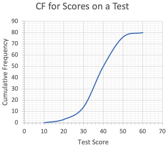
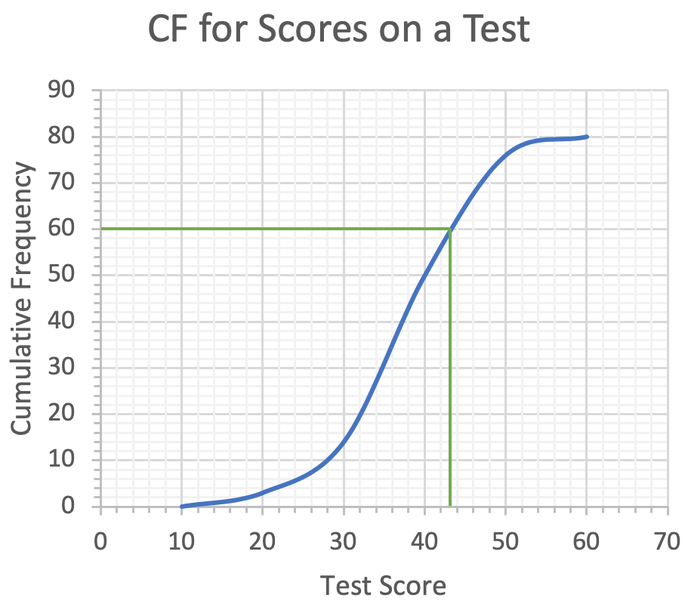
Below is a cumulative frequency graph for the test results for 80 pupils. What is the median, lower quartile, upper quartile and inter quartile range for the data below? Click here here for a printable version of the graph.


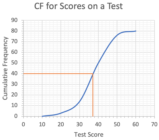
The median is the 40th term. We find the median by finding 40 on the cumulative frequency, going across to the curve and reading down to find the test score. The working is shown below.
The next step is to find the lower and upper quartile. The lower quartile is the median of the lower half of the data; it is the 25% value. The upper quartile is the median of the upper half of the data; it is the 75% value.
To obtain the term that is the lower quartile, we divide the number of values by 4. There are 80 values, so we divide 80 by 4. We divide by 4 because 25% is a quarter.
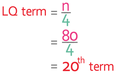
The lower quartile is the 20th term. We find this term by reading across from 20 on the cumulative frequency axis to the curve and then reading down to find the test score. The working is shown below.
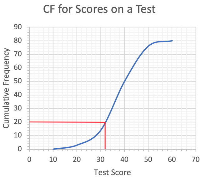
The lower quartile is 32.
To obtain the upper quartile, we multiply the number of values by 3 and then divide by 4. We multiply by 3 and divide by 4 because 75% as a fraction is 3/4.
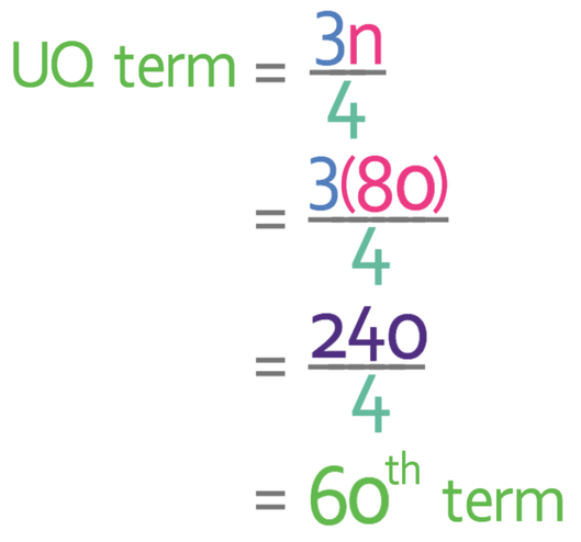
The upper quartile is the 60th term. The working is shown below.
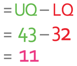
We are now able to work out the interquartile range and we do this by using the formula below:

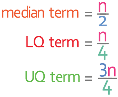
Here are the key formulas for working the term out for the median, lower quartile and upper quartile. n in all of the formulas is the number of values (for the above example, n was 80).

Sometimes it may be the case that the upper quartile is referred to as Q3 and the lower quartile is referred to as Q1. When this is the case, the formula for working out the interquartile range becomes:

The median is sometimes referred to as Q2.
There is more information on interquartile range in the analysing data section (6.3). Click here if you would like to be taken this section.