Back to Edexcel Analysing Data (H) Home
6.3 J) Analysing Grouped Data
6.3 J) Analysing Grouped Data
We are now going to have a look at finding the mean, mode and median from grouped data. Grouped data is often used for continuous data. Continuous data is numerical data that can take any value. For example, suppose that we were to measure the exact ages of the individuals that are watching a film at the cinema. We will likely get many different ages and our table will be very complicated and hard to understand. Therefore, we split the data into groups to make it easier to interpret.
Grouped data usually uses inequalities and this is because you need to make sure that every value appears in one and only one group. With our ages example, let’s suppose that everyone was under 50. We could split the ages that we have into 5 different groups. Only one end of the inequality should be inclusive (equal to). I am going to make the top end of my inequality inclusive. The groups that we could have could be:
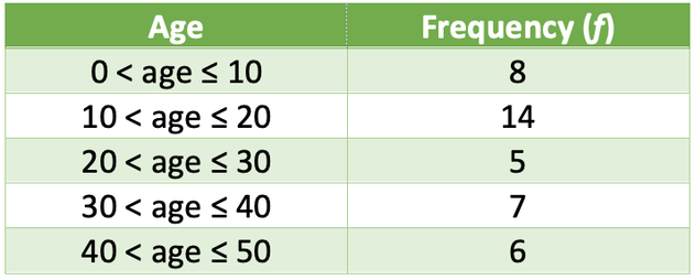
Let’s now add some data to our example. The table below shows the ages of individuals that went to the cinema to see a particular film.
Grouped data usually uses inequalities and this is because you need to make sure that every value appears in one and only one group. With our ages example, let’s suppose that everyone was under 50. We could split the ages that we have into 5 different groups. Only one end of the inequality should be inclusive (equal to). I am going to make the top end of my inequality inclusive. The groups that we could have could be:
- 0 < age ≤ 10
- 10 < age ≤ 20
- 20 < age ≤ 30
- 30 < age ≤ 40
- 40 < age ≤ 50
Let’s now add some data to our example. The table below shows the ages of individuals that went to the cinema to see a particular film.
A downside of receiving data that has already been organised into groups is that we do not know what the exact values are. This means that we are unable to find the exact value for the mean, mode and median. However, we are able to find an estimate for the mean, the modal group and the group that the median is in.
Modal Group
The modal group is the group that contain most of the values; it is the group with the highest frequency. We can see that highest frequency in the table is 14, which is the group 10 < age ≤ 20. Therefore, the modal group is 10 < age ≤ 20.
The modal group is the group that contain most of the values; it is the group with the highest frequency. We can see that highest frequency in the table is 14, which is the group 10 < age ≤ 20. Therefore, the modal group is 10 < age ≤ 20.
Group that Contains Median
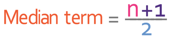
The median is the middle value and we are now going to look for the group that contains the median. We won’t be able to give the exact value of the median because we do not know the exact values for the data, but we can find the group that the median will be in. The median value is the middle term in the ordered data. We find what term the median is by adding 1 to the number of values that we have and dividing by 2.
The median is the middle value and we are now going to look for the group that contains the median. We won’t be able to give the exact value of the median because we do not know the exact values for the data, but we can find the group that the median will be in. The median value is the middle term in the ordered data. We find what term the median is by adding 1 to the number of values that we have and dividing by 2.
We are able to find the amount of values by adding all of the frequencies together.
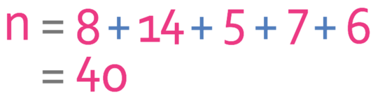
There are 40 values in the data set. Therefore, we sub n as 40 into the formula to find what term the middle term is.
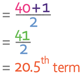
Therefore, we are looking for the 20.5th term, which is half away between the 20th and the 21st term. An easy way to find the group that contains this term is to add another column to the data that looks at cumulative frequency. Cumulative frequency is the sum of the frequencies for the class and all of the other classes below it in a frequency distribution. The cumulative frequency is shown in the table below.
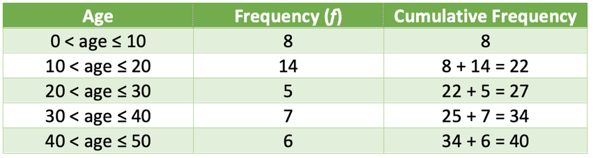
From the cumulative frequency column, we can see that the second group (10 < age ≤ 20) contains the 9th to the 22nd term. This means that the 20th and the 21st term (and therefore, half away between this term; the 20.5th) will be found in the second group. Therefore, the median is in the group 10 < age ≤ 20.
Estimated Mean
The mean is calculated by adding all of the values in the data set and dividing by the number of values. The formula is shown below:
The mean is calculated by adding all of the values in the data set and dividing by the number of values. The formula is shown below:

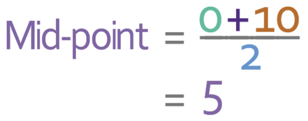
However, with grouped data, we do not have the exact values for the data because the values that have been placed into groups. This means that we cannot work out the exact mean for the data. But, we are able to work out an estimate for the mean by creating an estimate for the sum of all of the pieces of data. To find the estimate for the sum of all of the values, we create a new column for the midpoint for each of the groups. Usually you can see what the midpoint of the classes are by just looking at them. However, if you cannot see the midpoint straight away, you add the numbers at the start and the end and then divide by 2. Let’s work out the midpoint for the first group:
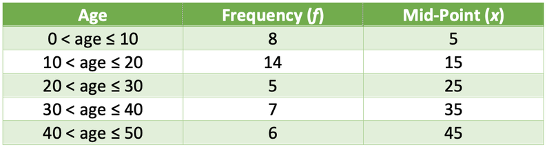
The table below shows mid-points for the 5 groups in the table.
The next step is to multiply the frequency (f) by the mid-point (x).
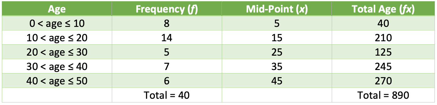
For the mean, we need to know what the sum all of the values are (which for this example is the sum of the ages) and the amount of values (the total number of people asked/ involved). We are now able to find an estimate for the mean.
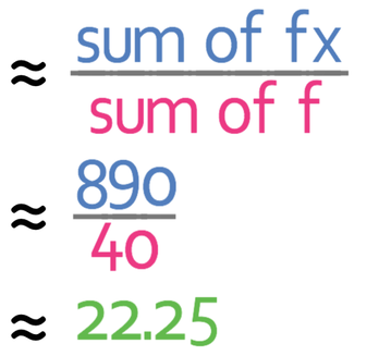
The estimated mean ages of the individual in the cinema is 22.25 years.