Back to OCR Linear Graphs (F) Home
2.5 D) Plotting Linear Graphs
2.5 D) Plotting Linear Graphs
In the previous section we looked at modifying equations for graphs to get them into the form y = mx + c. One reason for doing this is so that we can quickly see the gradient (the value of m) and the y intercept (the value of c) for the graph. A second reason for getting graphs into the form y = mx + c is because graphs are considerably easier to plot/ find the coordinates when they are in this form.
In order to plot linear graphs, we sub a few different x values into the equation to find the respective y values. This gives us the coordinates, which we can then plot on a graph. We then draw a line through all of the coordinates; we need to continue the line past the end coordinates rather than ending the line at the coordinates.
In order to plot linear graphs, we sub a few different x values into the equation to find the respective y values. This gives us the coordinates, which we can then plot on a graph. We then draw a line through all of the coordinates; we need to continue the line past the end coordinates rather than ending the line at the coordinates.
Plotting Example 1
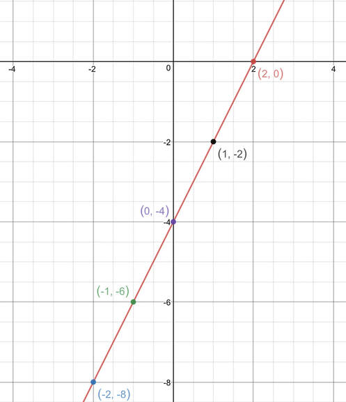
Plot the equation y = 2x – 4.
I am going to sub 5 different x values into this equation and I am going to use a table to help me. Every table that we use will have the rows “x value”, “y value” and “coordinates”. The other rows in the table will depend on the equation that we are plotting. We are plotting y = 2x – 4. We are going to have another row for each of these components.
We then find the y values by adding the values in the 2x row to the values in the -4 row. To find the coordinates, we take the x value that we subbed in and the y value that we got out.
Plot the equation y = 2x – 4.
I am going to sub 5 different x values into this equation and I am going to use a table to help me. Every table that we use will have the rows “x value”, “y value” and “coordinates”. The other rows in the table will depend on the equation that we are plotting. We are plotting y = 2x – 4. We are going to have another row for each of these components.
- We will have a row for 2x, which will be where we multiply the x value by 2. The values along this row will be different because the value of 2x is dependent on the value of x that we are subbing in.
- The next row will be -4, which will be the same across the whole row.
We then find the y values by adding the values in the 2x row to the values in the -4 row. To find the coordinates, we take the x value that we subbed in and the y value that we got out.
The next step is to plot the coordinates at the bottom of the table and draw a line through the points (it is important that we continue the line through the start and end of the points rather than stopping on the points that are furthest out).
Plotting Example 2
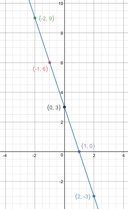
Plot the equation y = -3x + 3.
Like the question before, I am going to be using a table to find a few coordinates for this graph. We will have the standard 3 rows in the table; “x value”, “y value” and “coordinates”. The other rows in the table will depend on the equation that we are plotting. I am plotting y = -3x + 3, which means that I will have a -3x row and +3 row. The filled out table is given below.
We now plot the coordinates at the bottom of the table and draw a line that passes through all of the points (make sure that the line that you draw continues past the points at the end of the line). The graph is plotted below.


