Unstable atoms emit radiation so that they become stable. The emitting of radiation from atoms is known as radioactive decay. We can measure the amount of radiation that a substance is giving off by using a Geiger-Muller tube and counter, which detects all of the different types of radiation. The GM counter measures the quantity of radiation per second, which is referred to as the activity or count rate. We measure the count rate in becquerels (Bq) where 1 Bq is 1 decay per second.
Radioactive decay is a random process and is not affected by physical conditions. This means that we cannot predict when a particular atom will undergo radioactive decay. Instead, we work out the time that it takes for half of a radioactive material to decay. This is known as the half-life of a radioactive isotope. A half-life is the average time that it takes for the number of radioactive nuclei in an isotope sample to halve.
For example, let’s suppose that I have a sample that contains 400 radioactive isotopes.
So, we started with 400 radioactive isotopes and after 1 half-life had 200 that were still radioactive, and after 2 half-lives had 100 that were still radioactive and after 3 half-lives had 50 that were still radiative etc.
All of the half-lives for the above sample will be the same length of time. For example, if the half-life for our sample was 6 days, the first half-life would be 6 days, the second half-life would also be 6 days, the third half-life would also be 6 days etc.
As a radioactive sample decays/ more half-lives occur, the number of radioactive atoms in the sample decreases. This means that there will be fewer atoms undergoing radioactive decay and therefore, less radiation being emitted. This will mean that the count rate will decrease as the sample decays/ more half-lives occur (count rate is measured by a Geiger-Muller tube and it is measured in becquerels (Bq); count rate is also known as activity).
Radioactive decay is a random process and is not affected by physical conditions. This means that we cannot predict when a particular atom will undergo radioactive decay. Instead, we work out the time that it takes for half of a radioactive material to decay. This is known as the half-life of a radioactive isotope. A half-life is the average time that it takes for the number of radioactive nuclei in an isotope sample to halve.
For example, let’s suppose that I have a sample that contains 400 radioactive isotopes.
- After one half-life, half of these 400 isotopes will have decayed. This means that 200 of the isotopes have decayed and are now stable, and 200 isotopes are still radioactive.
- After a second half-life, half of the now 200 radioactive isotopes will have decayed, which means that 100 of the isotopes will have decayed and become stable, which leaves 100 isotopes that are still radioactive.
- After a third half-life, half of the now 100 radioactive isotopes will have decayed, which means that 50 will have decayed and become stable, which leaves 50 isotopes that are still radioactive.
So, we started with 400 radioactive isotopes and after 1 half-life had 200 that were still radioactive, and after 2 half-lives had 100 that were still radioactive and after 3 half-lives had 50 that were still radiative etc.
All of the half-lives for the above sample will be the same length of time. For example, if the half-life for our sample was 6 days, the first half-life would be 6 days, the second half-life would also be 6 days, the third half-life would also be 6 days etc.
As a radioactive sample decays/ more half-lives occur, the number of radioactive atoms in the sample decreases. This means that there will be fewer atoms undergoing radioactive decay and therefore, less radiation being emitted. This will mean that the count rate will decrease as the sample decays/ more half-lives occur (count rate is measured by a Geiger-Muller tube and it is measured in becquerels (Bq); count rate is also known as activity).
Half-Life Graph
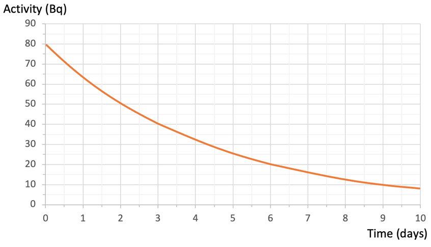
We can draw a graph that shows the activity (count rate) of a radioactive isotope against time; activity (count rate) is plotted on the y axis and time is plotted on the x axis. An example of a half-life graph is shown below:
We can draw a graph that shows the activity (count rate) of a radioactive isotope against time; activity (count rate) is plotted on the y axis and time is plotted on the x axis. An example of a half-life graph is shown below:
Question 1
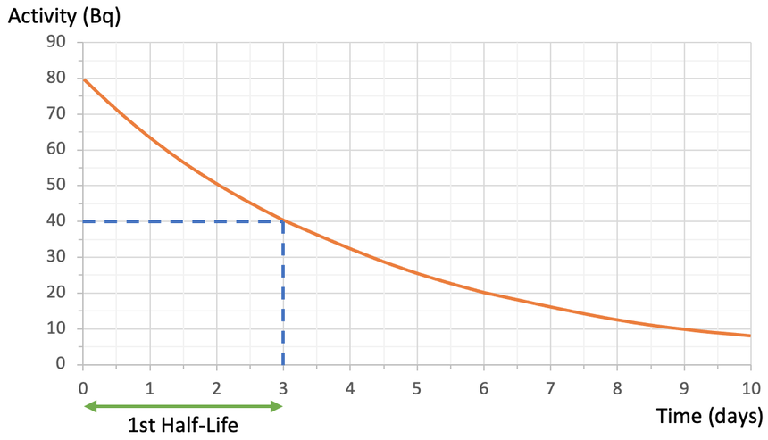
Using the graph above, find the length of a half-life.
The radioactive isotope has an activity of 80 Bq at the start. After one half-life, half of the radioactive substance will have decayed, which means that the count rate will be half of what it originally was. The original count rate was 80 Bq, so after 1 half-life, the count rate will be 40 Bq (½ x 80 = 40). Therefore, we find 40 Bq on the y axis and read across to the curve and down to the x axis to find the time. When we do this, we see that it takes 3 days for the activity of the radioactive substance to half. Therefore, the half-life for this substance is 3 days.
The half-life for a substance will always be the same and this is because radioactive decay is a completely random process. Therefore, the half-life for this substance will always be 3 days.
This means that the second half-life for this substance will take another 3 days (the second half-life will have happened after 6 days). After the second half-life, the activity will be half of what it was after the first half-life. After the first half-life, the activity was 40 Bq. After the next half-life, the activity will be half of this, which means that the activity will be 20 Bq (½ x 40 = 20). So, after the second half-life, we will have a count rate of 20 Bq and it will occur at 6 days.
This means that the second half-life for this substance will take another 3 days (the second half-life will have happened after 6 days). After the second half-life, the activity will be half of what it was after the first half-life. After the first half-life, the activity was 40 Bq. After the next half-life, the activity will be half of this, which means that the activity will be 20 Bq (½ x 40 = 20). So, after the second half-life, we will have a count rate of 20 Bq and it will occur at 6 days.
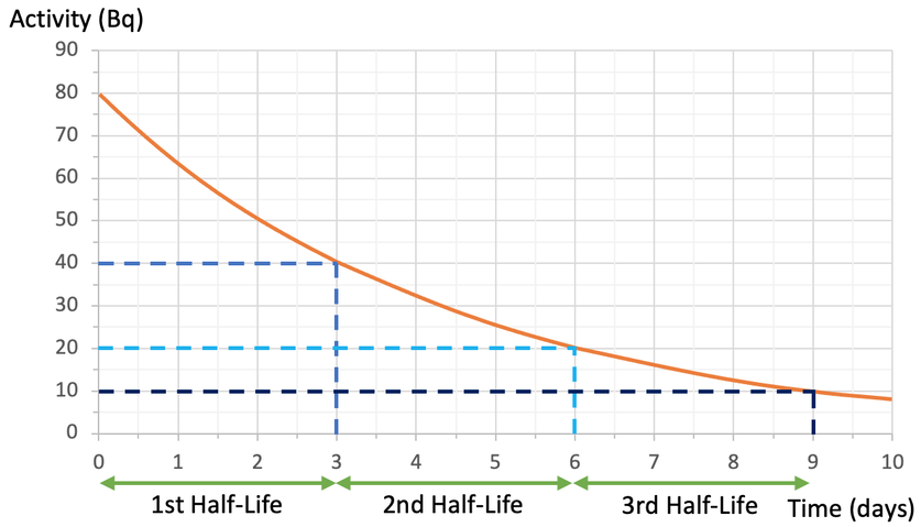
The third half-life will take another 3 days (it will happen at 9 days) and the activity will be 10 Bq (½ x 20 = 10). This is shown on the above graph.
Half-Life Times
The time taken for different radioactive isotopes to decay varies a great deal. For some substances, the half-lives can be a few seconds and for other substances the half-lives can be millions of years. For example, the half-life of silver-110 is 24.6 seconds, the half-life for carbon-14 is 5,700 years and the half-life for uranium-238 is 4,460,000,000 years (you do not need to remember any of these for the exam; they are just here to show you that the half-lives for different radioactive isotopes vary a great deal).
A short half-life means that the nuclei decay quickly, meaning that the activity falls quickly. A long half-life means that the nuclei decay slowly, resulting in the activity falling at a slower rate.
Question 2
We have an initial activity of 1,200 Bq for a radioactive substance (francium-223). The half-life of francium-223 is 20 minutes. What will be the activity after 80 minutes?
The first step is to work out how many half-lives will occur during the total time period. The total time period is 80 minutes and one half-life is 20 minutes. We work out the number of half-lives by dividing the total time period (80 minutes) by the length of a half-life (20 minutes).

This tells us that in 80 minutes, there will be 4 half-lives.
We can now work out the activity of the radioactive substance by halving the initial activity (1,200 Bq) 4 times.
We can now work out the activity of the radioactive substance by halving the initial activity (1,200 Bq) 4 times.
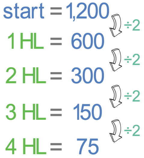
Therefore, at the end of the 80 minutes, the activity rate will be 75 Bq.
Question 3
Find the time for one half-life on the graph below.
Find the time for one half-life on the graph below.
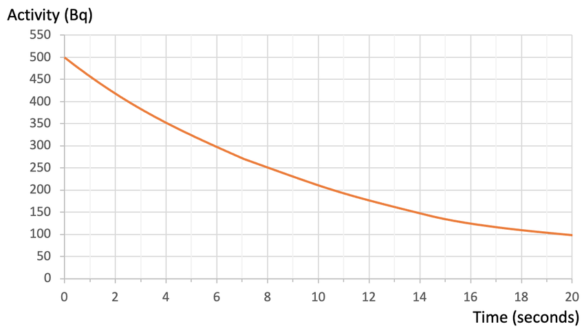
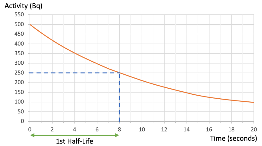
The activity for the radioactive substance at the start was 500 Bq. After 1 half-life, the activity will be half of what it was at the start. This means that the activity after 1 half-life will be 250 Bq (½ x 500 = 250). We find the length of 1 half-life by reading across from an activity of 250 Bq on the y axis to the curve, and then down to the x axis. When we do this, we see that the length of time for a half-life is 8 seconds (the working is shown below)
Question 4
We are now going to have a look at a question whereby we are asked to draw a graph showing how the activity of a radioactive substance changes over time. When we are given a question like this, we will be given the initial count rate/ activity and the length of time for a half-life.
Question
The initial activity for a radioactive substance is 160 Bq. The half-life for this substance is 6 years. Draw the graph showing how the activity for this radioactive sample varies over time.
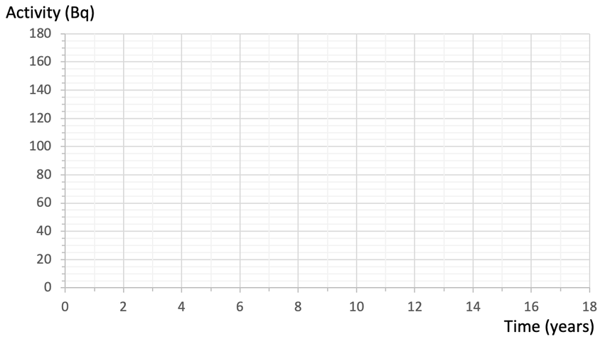
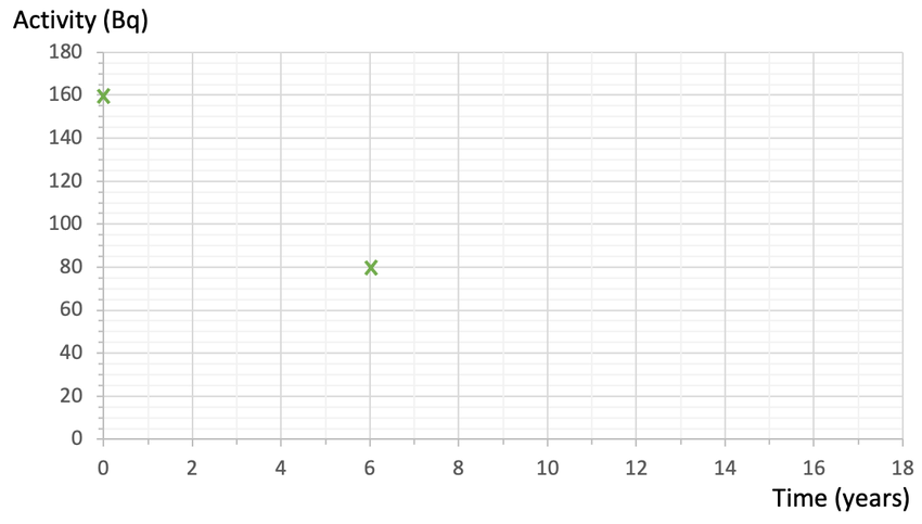
We are told in the question that the initial count rate is 160 Bq. Therefore, the first step is to mark 160 Bq and a time of 0 onto the graph.
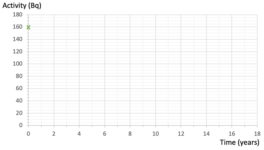
After 1 half-life, the activity of the radioactive substance will be half of what it originally was. The original activity was 160 Bq, which means that after 1 half-life, the activity will be 80 Bq (½ x 160 = 80). The question tells us that a half-life for this substance takes 6 years. Therefore, the second point that we mark on the graph is a time of 6 years and an activity of 80 Bq.
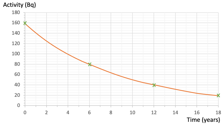
We now find the values after the second half-life. The activity after the second half-life will be half of the activity after the first half-life; the activity after the second half-life will be 40 (½ x 80 = 40). The time after the second half-life will be another 6 years, which means that the second half-life occurs after 12 years (6 + 6 = 12).
We now find the values after the third half-life. The activity after the third half-life will be half of the activity after the second half-life; the activity after the third half-life will be 20 (½ x 40 = 20). The time after the third half-life will be another 6 years, which means that the third half-life occurs after 18 years (12 + 6 = 18).
We plot the values for the second and third half-life onto the graph and draw a smooth curve passing through the 4 points.
Questions like this can be extended by being asked to estimate the activity after a certain period of time. For example, estimate the activity from this radioactive sample after 10 years.
We can estimate the activity after 10 years by finding 10 years on the x axis, reading up to the curve and then across to the y axis. The working for this is shown on the graph below.
We can estimate the activity after 10 years by finding 10 years on the x axis, reading up to the curve and then across to the y axis. The working for this is shown on the graph below.
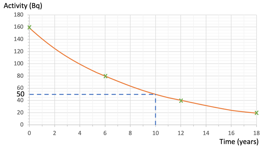
From our working, we can see that an estimate for the activity after 10 years is 50 Bq.
Question 5
The next question has been taken from a past paper.
Question
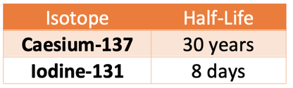
The table below shows the half-lives of two of the radioactive isotopes that contaminated the environment after the Chernobyl disaster in 1986.
The next question has been taken from a past paper.
Question
The table below shows the half-lives of two of the radioactive isotopes that contaminated the environment after the Chernobyl disaster in 1986.
A soil sample was taken from the area around Chernobyl in 1986
The soil sample was contaminated with equal amounts of caesium–137 and iodine–131
Both isotopes emit the same type of radiation.
Explain how the risk linked to each isotope has changed between 1986 and 2018
Answer
The amount of time between 1986 and 2018 is 32 years.
Let’s start by looking at caesium-137. The half-life of caesium is 30 years (quite a long time), which means that over the 32 years between 1986 and 2018, just over 1 half-life will have happened. Therefore, there will still be a lot of radioactive caesium-137 in the soil sample in 2018, which means that the caesium-137 will have a high activity and still have a high risk.
Let’s now have a look at iodine-131. The half-life of iodine-131 is 8 days (a very short time), which means that there will have been many half-lives in the 32 years between 1986 and 2018. Therefore, there will be very little radioactive iodine-131 in the soil sample in 2018, which means that iodine-131 will have a low activity and a low risk.
So, there will be a high risk from caesium-137 as it has a long half-life, and a low risk from iodine-131 as it has a short half-life.